

Two Great Reads - Monday - December 2
Siblings!

Today we’re going to take deep dives into two methods-ish articles that ask us to think seriously about how to handle datasets that include sibling pairs.
The articles reviewed today are the kind that I absolutely love. They are examples of highly sophisticated thinking that deploy interesting causal and/or statistical techniques - e.g., the use of directed acyclic graphs or variance decomposition. Yet both ask you to do the hard work of thinking about your darned data and your research question. Broadly speaking, there are two directions that methods paper go - (1) the goal of a quantitative social science paper should be maximal complexity to match the complexity of the data (2) complexity above and beyond a simple comparison of means represents a failure of research design and/or the nature of the data, and so we must think carefully about when and why we introduce complexity and consider that application as a loss. Perhaps you can tell in my descriptions that I am a big fan of the logic of (2), and both of these papers are sterling examples of methods paper (2) logic.
Sibling data
Before we start, let’s sketch out sibling data. Think about two types of datsets. Dataset one wishes to collect a population representative sample of individuals in the US population. Therefore, researchers randomly call up landline and cellphone numbers and collect a sample of 1,500 individuals. It is possible, but very unlikely, that any two people randomly called up will be siblings. The observations will be independent and identically distributed - e.g. if two siblings end up in your sample, that’s just the outcome of random probability. Dataset two randomly samples to collect a population representative sample of families. So, for example, you might call me up, learn that I have a daughter and son, collect information about them, and track the two of them into adulthood.
The nice feature of the sibling data structure is that you can account for a large variety of important but difficult-to-measure features of family background. Let’s say that you’re interested in how a person’s education affects their earnings. There are lots of reasons why two random people with different levels of education differ - reasons which are difficult to collect in a survey. The broad logic of sibling datasets is that you can compare differences in education and earnings within sibling pairs - you account for lots of important background features of individuals if you look at these within sibling differences (e.g. my sister attained more education and is more economically successful than me is a more meaningful comparison than my sister attained more education and is more economically successful than some random other American).
A caution on sibling comparisons in studying effects of the rearing environment
Engzell and Hallsten (EH) wrote an amazing article that challenges the thoughtless application of sibling comparisons. The motivation:

EH ask us to think of two types of sibling comparisons: in one, both the treatment and the outcome stem within the sibling (e.g. one sibling happened to see the Nutcracker on PBS, developed a love of ballet, and started sneaking to the Met on the weekend, the other sibling didn’t), and aren’t due to the parents. But EH notice that lots of studies using sibling comparisons are using parent-level characteristics as the treatment (e.g. parents take one of their kids to the ballet, not their other kid).

EH sketch out these two types of sibling comparisons:

Notice where the treatments, E, come from: differences across the siblings themselves (left diagram) or different treatment by parents (the right panel). The right diagram - discordant family design (DFD) - can cause theoretical issues.
The problem with DFD is subtle, but important. We’re almost always interested in between family comparisons - e.g. does growing up in a rich versus poor family affect a child’s outcome, does growing up in a house with and without books increase a child’s educational attainment. The DFD approach assumes equivalence of within-family and between-family effects: e.g. a family with books is the same as a family buying five more books. If you think about it for a hot second, that’s an unrealistic assumption.
EH go a bit more in depth on these assumptions. Look at their Figures 2 and 3.

If variation across siblings comes from the siblings themselves and not their families, then we’re in Figure 2 world, and things work ok. But if we’re using DFD logic, we are making the assumption in Figure 3. That is, that the thing we can’t observe, U, affects time-stable between-family effects, E_j, which affects the variation of parent treatment of children, E_ij, which affects the outcome we care about. That is, all parent effects occur through differential treatment of their children. EH say, let’s write out ways that such an assumption might not work.
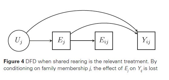
Figure 4 says - maybe differential treatment of children isn’t that important. Maybe it’s the similar treatment of children that matters. Their description of Figure 4:


My understanding: perhaps you’re interested in parenting style on children’s school behavior. I do actually treat my children slightly differently. But I coddle and helicopter over them both. That similar parenting style might be the fundamental reason why my kids act at school in one way, whereas my friend Jo’s free-range parenting style influences their kids’ school behavior.
Furthermore, maybe the variation across siblings is due to something other than time-stable parent characteristics!

EH’s interpretation

My understanding: (1) one of my child has autism, which affects both how I treat that child at home, and how they behave at school. My differential treatment between child 1 and 2 does not cause variation in behavior. (2) My kid has a naughty friend who motivates them to put a whoopie cushion on their teacher’s chair. I go to a parent-teacher meeting, and I start treating this child more strictly afterwards. The other child was lucky to have angelic friends, and my treatment of them remains at baseline. My differential treatment of children responds to behavioral differences, undercutting the DFD approach.
EH then run through a few examples from the literature:
Parenting style. How likely is it that parents take one of their children to the museum and not the other? Not terribly likely. This gets even worse when we use twins, as spacing of children might take out any form of change in parenting style over time.
Income. When we use the DFD approach, we’re really measuring the effect of “transitory” income, instead of “permanent” income (e.g. the random fluctuation of your pay between 2019 and 2022, rather than the fact that your HR job pays more than another’s taskrabbit job). This is a problematic selection, since most theories would suggest that permanent income would be more consequential.
Neighborhood effects. Where you grow up matters, but neighborhood effects should be more durable and cumulative:

EH note that some folks try to salvage the DFD approach by using panel data (e.g. tracking siblings over time). But EH say: doesn’t that really just shift our research design to a within-person one?

EH’s recommendation:

They ask we consider 7 questions before going down the sibling comparison route:


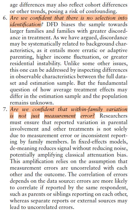
I’d summarize these as: why are you doing this study? What are you trying to accomplish? Did you stop for a hot second to think about what you’re doing?
Really good study. I freaking love these types of articles that ask you to think seriously about what you’re doing.
Decomposing sibling correlations: a new measure of group-specific intergenerational persistence in socioeconomic outcomes

I wrote about a similar article a few months back, but I thought I’d dive into this recent article.
It provides a very cool and surprisingly simple trick to examine where sibling correlations come from.
Let’s think about a dataset with sibling pairs:

We have 8 people here, and people are nested in four sibling pairs (differentiated by highlighted groups and the SiblingPair column). Siblings have particular incomes. We can roughly break apart the total income into three components:

TotalMean, FamilyIncome, and IndividualResid are (1) the overall mean income (2) the family component of income (e.g. how much family groups share being above or below the overall mean income) and (3) sibling variation (e.g. how much siblings are different from their family-specific difference from the overall mean).
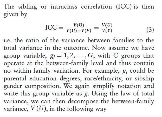
(2) and (3) are the really cools parts, because they let us construct something called a sibling intraclass correlation, or the percent of the variation of our outcome that is due to component (2):
In our example, the ICC is 0.89 - 89% of the variation of our pretend income variable is due to differences between families, while 11% of the variation of our pretend income variable is due to differences between siblings within families.
Just to hammer this point - here are two pretend incomes.
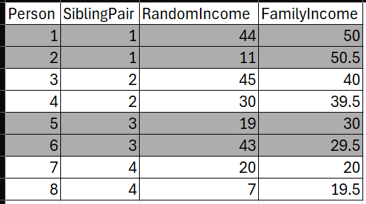
RandomIncome has an ICC of 0.44 - there’s less differences between families than there is between siblings within families. FamilyIncome has an ICC of 0.99 - almost all the differences in income are between families.
ICC is cool because it gives you a simple descriptive measure of variation in the outcome that is due to family differences.
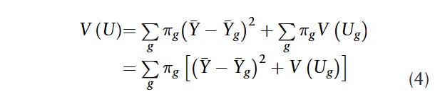
What Karlson an In (KI) do is really neat. They say - hey: ICC is really just a ratio of variances, and there are well-established techniques of variance decomposition that can be spun out to get a bit of a sophisticated understanding of who’s responsible for a particular ICC level. Let’s decompose this family component of ICC into contributions across distinct groups:
Group, g? Well, think of that as siblings whose father is Black and siblings whose father is White. Or think of it as siblings whose mother has a college degree, and siblings whose mother does not. Or sibship pairs: two brothers (group 1), two sisters (group 2) and a brother and sister (group 3). We can see how much of the overall ICC is driven by each of these groups.
There are three important chunks in this variance decomposition:

This is the weight - or the percentage of the sample that is in each of the group.

This is the group-specific mean, compared to the overall sample mean. e.g. children whose parents have a college degree have relatively high incomes. Children whose parents don’t have college degrees have relatively lower incomes.

The group-specific variation. e.g. does family do a lot to explain earnings among those whose mother has a college degree?
We can basically end up looking at the overall ICC as a weighted fraction of the sum of chunks two and three, letting us determine which groups are driving the overall ICC:

KI also go on to show how this decomposition lets us better understand changes over time by (1) looking at the same groups across two time periods (e.g. 30 year olds in 2004 and 30 year olds in 2024), fixing one of the three chunks in the latter time period to the value in the earlier time period (e.g. holding the % of children from college educated backgrounds in 2024 at their 2004 levels), and then assessing how much the overall ICC changes.
KI then go on to a few substantive examples. They use the NLSY79 dataset, which tracks a cohort of folks over time who were roughly 14 in 1979. This dataset includes information of sibling pairings, and KI examine the ICC of earnings age 30 and onward from brother pairs, stratified across four income groups (e.g. parents in the bottom 1/4, bottom middle 1/4, top middle 1/4, top 1/4 of the parent income distribution).

The overall ICC is 0.41 (e.g. about 40% of the variation of adult incomes occur across families, while about 60% of variation of earnings occurs across brother pairs, circled in red).
That 0.41 isn’t evenly distributed across parent income origin. If you at the numbers circled in blue, you see that the big family payoff comes from Q4, or the highest income origins. This is driven both by this group’s higher mean pay (0.231), and by the fact that family is more predictive of both sibling’s earnings (0.281).
They also look at ICCs across brother-brother, sister-sister, and brother-sister pairings in the NLSY79

The ICC here is 0.22 (makes sense of lower family similarity when women during the 2nd wave of feminism are included).
Over half, 55% in the blue circle, of this family component comes from brother-brother pairs. And a big chunk of this, 0.287, comes from the family-predictiveness across brother pairs.
It’s a simple, but very clever and cool, way to unpack why between family characteristics matter, and how to identify which groups are more consequential for family similarity.
Miscellaneous thoughts
Both of these papers do a great job inching you toward thinking about your data. “Why would I use sibling comparisons?” “Why would parent treatment vary across siblings?” “Why would family effects be larger in one group versus another?” At a basic scholarly level, that’s incredibly important.
At a more pragmatic level, knowing your data and thinking deeply about your data doesn’t help you address a modern form of reviewer, which I sometimes jokingly call the “But Causal” reviewer. Such a reviewer will sometimes have one thing to say: “This study isn’t causal,” or “The association is descriptive, not causal,” etc. To be honest, I’ve been a “But causal” reviewer before. Sometimes it’s an important critique. But other times you’ve thought deeply about your research question, sketched out a sophisticated description such as EH and KI recommend, and describe the limitations of your approach. Some studies are necessarily descriptive, and the goal is to be thoughtfully descriptive. And you’ll get a But Causal reviewer who says, “This study isn’t causal.” Sadly, one effective method to combat a more hurried and inattentive But Causal reviewer is to take EH’s DFD approach, say, “Identified, Is Causal,” which often satisfies the modal But Causal reviewer. Then your paper adds to the problem identified by EH, and cannot address the cool between family issues pointed to by KI. This is all to say: EH and KI are recommending you think seriously and have humility about your research design. But that also requires you get three reviewers who think seriously and understand the humility required to address important sociological questions. You’ll rarely find that in the wild, which makes the approaches proposed by EH and KI a bit risky to implement by themselves.